Phase 1 calibration study¶
These are the first numbers this project can honestly call its own. Everything here is
measured against the ground-truth fake client (testing/fake.py), the only place where a
node's true bias is known. Nothing here is a claim about real models or published benchmarks.
Reproduce:
Raw results: phase1-results.json. Figures: figures/. Full run: 300 unbiased nodes for calibration, 120 per sensitivity/budget point, 80 for estimator agreement; 400 permutations and 200 bootstrap resamples per score; seed 20260731.
Headline findings¶
- The detector is well calibrated. On unbiased nodes the permutation p-value is uniform and the false-positive rate tracks the nominal α across every sampling-noise level tested. This is the property that makes the whole system falsifiable, and it holds.
- Detection floor ≈ β 1–2 at the default budget (n=8, noise=0.6): bias of magnitude β=2 is caught with 97% power, β=1 with ~48%, and below β=0.5 detection is near the noise.
- The real cost multiplier is
n × (1 + axes)— roughly 10–32× at usable settings, not the 3–6× estimated in DESIGN.md. This is the most important operational finding and it directly justifies centrality-scaled probing and null-caching before any production use. - Effect size is not comparable across sample budgets. It is a standardized detection statistic that inflates with n (same β=2 bias reads as 1.9σ at n=3 but 22.9σ at n=30), so M2 must hold n fixed or weight on an n-stable magnitude instead.
- CHOICE and GENERATIVE agree only moderately (Spearman ρ≈0.56). The embedding path is a real but noisier signal, consistent with calling it a semantic proxy rather than a calibrated divergence.
1. Calibration — false positives are controlled¶
On unbiased nodes, a permutation test should yield p ~ Uniform(0,1); then the false-positive rate at threshold α is exactly α. It does. Mean p-value stays at ≈0.50 across all noise levels, and the empirical CDF lies on the diagonal.
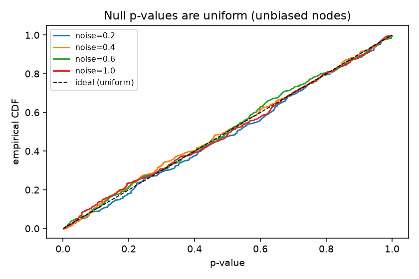
| sampling noise | mean p | FPR @0.01 | FPR @0.05 | FPR @0.10 |
|---|---|---|---|---|
| 0.2 | 0.512 | 0.007 | 0.050 | 0.090 |
| 0.4 | 0.491 | 0.003 | 0.047 | 0.110 |
| 0.6 | 0.492 | 0.013 | 0.060 | 0.107 |
| 1.0 | 0.498 | 0.010 | 0.067 | 0.123 |
FPR at α=0.05 ranges 0.047–0.067 (target 0.05) — within sampling slack for 300 trials. Crucially, this holds whether the node is nearly quiet (noise 0.2) or very noisy (noise 1.0): the noise floor is doing its job of subtracting sampling variance rather than flagging it as bias.
2. Sensitivity — how much bias is detectable¶
Injected bias magnitude β vs. recovered effect size and detection power (α=0.05, n=8, noise=0.6):
| β | mean effect size | power |
|---|---|---|
| 0.0 | 0.01 | 0.033 |
| 0.25 | 0.24 | 0.092 |
| 0.5 | 0.52 | 0.125 |
| 1.0 | 2.12 | 0.483 |
| 2.0 | 5.75 | 0.967 |
| 4.0 | 9.00 | 1.000 |
| 8.0 | 10.77 | 1.000 |
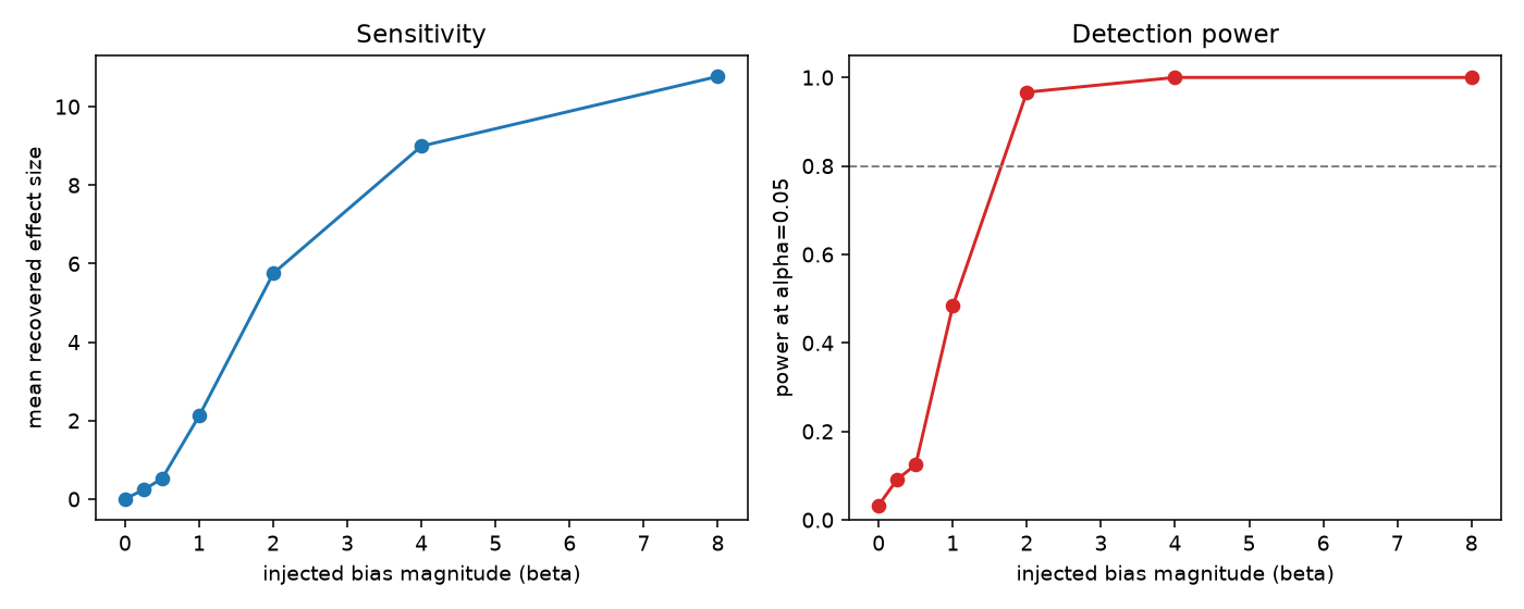
Effect size rises monotonically with β (the WP1 fake contract in action), and power crosses the conventional 80% line between β=1 and β=2. Detection floor at the default budget: β≈2. Subtle bias (β≤0.5) is at the edge of the noise and needs a larger sample budget to see (§3). At β=0 the power is 0.033 — i.e. the false-positive rate again, consistent with §1.
3. Sample budget — what precision costs¶
Fixing β=2.0 and varying samples per side (n):
| n | mean effect size | mean null σ | power | calls (1 axis) |
|---|---|---|---|---|
| 3 | 1.88 | 0.0325 | 0.000 | 6 |
| 5 | 3.37 | 0.0195 | 0.825 | 10 |
| 8 | 5.93 | 0.0131 | 0.958 | 16 |
| 12 | 9.15 | 0.0091 | 1.000 | 24 |
| 20 | 15.47 | 0.0053 | 1.000 | 40 |
| 30 | 22.88 | 0.0035 | 1.000 | 60 |
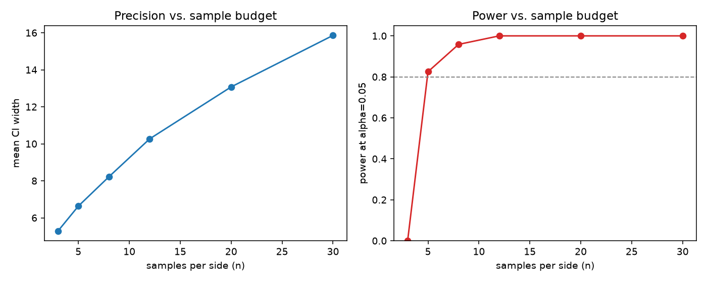
n=3 is unusable (0% power — too few samples for the permutation null to resolve anything). Power becomes usable at n=5 (83%) and solid at n=8 (96%). This sets the practical minimum.
The table also exposes finding #4: as n grows, the null standard deviation shrinks (0.033 → 0.0035,
roughly ∝ 1/√n) while the true divergence stays fixed, so the standardized effect size inflates
without bound. The same β=2 bias reads as 1.9σ at n=3 and 22.9σ at n=30. Consequence for M2/M3:
effect size is a detection statistic, not a portable magnitude — do not compare or threshold effect
sizes computed at different n. Either fix n across the deployment, or have M2 weight on an
n-stable quantity (raw_divergence net of null_mean), to be validated when M2 is built.
4. Estimator agreement — CHOICE vs. GENERATIVE¶
Scoring the same nodes both ways (candidate JSD vs. embedding distance), Spearman rank correlation of effect sizes is ρ ≈ 0.56 over 80 nodes.
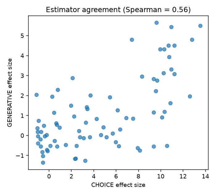
They agree on direction and broad ranking but not tightly. The embedding path carries a real
signal but a noisier one — which is exactly why the design treats GENERATIVE as a semantic proxy,
keeps the task_mode attached to every score, and forbids mixing the two scales. Do not expect a
GENERATIVE score to substitute for a CHOICE score on the same node.
5. Cost — the honest multiplier¶
An uninstrumented node makes 1 model call. A probe makes n × (1 + axes): n baseline resamples
(shared across axes) plus n per counterfactual axis.
| n | 1 axis | 2 axes | 3 axes |
|---|---|---|---|
| 5 | 10× | 15× | 20× |
| 8 | 16× | 24× | 32× |
At the usable minimum (n≥5) this is 10× for a single axis and 20–32× for multi-axis probing — well above the "doubles inference cost" / "3–6×" figures in DESIGN.md §2c, which are hereby corrected. Scoring CPU is negligible by comparison (~0.07s per axis for 400 permutations).
Implications, already in the roadmap:
- Centrality-scaled probing (M2) is not optional — full multi-axis probing of every node is
10–32× and will be switched off in production if applied uniformly.
- Null caching matters. The noise floor is a property of the node, not the input, so the n
baseline resamples can be amortized across many inputs, reducing marginal per-probe cost toward
n × axes (counterfactual-only).
- n=5–8 is the sweet spot: below it power collapses, above it cost grows for little power gain.
What this does and does not establish¶
Establishes (on the fake): the estimator is calibrated, monotonically sensitive with a quantified detection floor, has a known sample-budget/power curve, and a measured — not estimated — cost multiplier. The Phase 1 acceptance criteria are met.
Does not establish: anything about real models. The fake proves the estimator is correct; it cannot prove the estimator is realistic. Confirming that real LLM bias produces comparable curves — and that CHOICE and GENERATIVE agree on real outputs — is future work, explicitly not claimed here.